As technology buzzwords go, we think you’d be hard-pressed to find two that are more prevalent right now than neural networks and artificial intelligence; and with good reason. They are widely in use today, powering the image recognition in your favourite (or not so favourite) social media platform; the speech recognition systems on your intelligent connected speaker, and the digital voice assistant in your smartphone. The ability of neural networks to recognise patterns better than humans means they now help doctors identify cancers, assist farmers to improve their crops and identify people in a crowd. They’ll soon be found in embedded devices such as security cameras and with face recognition to unlock phones, they’ll increasingly be found in all our pockets.

However, to train a neural network requires powerful hardware and takes time and what can be run on a powerful server in the cloud can’t simply be ported to a mobile device due to their inherent limitations on computing and battery power.

Fortunately, there is a difference between training a neural network, ‘offline’ and the trained model that can recognise new objects in real time, known as ‘inference’. For example, if a neural network is designed to recognise that old image classification favourite, a cat, it will have learned what moggy looks like from a database of thousands of images of cats. Once appropriately trained, if you show a neural network powered device a picture of Mr Tiddles the cat, it will be able to recognise him even though it hasn’t seen him before. This is inferencing.

Demo of inferencing in action on the PowerVR Series2NX NNA

So when power and battery life are a concern, as they are for mobile devices, anyone creating a neural network application will want to train it in such a way as to optimise the inference stage as much as possible. This is done by reducing the computational complexity and bandwidth and as a result, save power.

This was the subject of a talk given by Paul Brasnett, Imagination’s Principal Research Engineer for vision and AI research, at the Embedded Vision conference earlier this year. You can view the whole thing at the EVA website, but you’ll need to be registered to do so.

So how is this achieved? In essence, optimising the network is done by shrinking down the trained neural network to make it easier to run by reducing redundancies. It’s similar in concept to how a digital image is commonly shrunk down from its uncompressed state to a space-efficient format such as a JPG. If the compressing algorithm is good, this can be done with very little appreciable difference in image quality. In neural network terms, image quality equates to inferencing accuracy. With suitable training, an optimised neural network can be greatly reduced in terms of size and complexity, all the while ensuring that the accuracy of the inferencing remains high.

Of course, not all networks are created equal. The first step will be to choose the best neural network model for your task. After all, if it’s not the most suitable, then even optimisation will not help you obtain the right results.

Eliminate, then reduce
Assuming you have the best model for your type there are two key stages to the optimisation process – elimination and then reduction.

First, you want to reduce the number of operations inside your network, and then you want to further reduce the compute cost of the operations that remain.

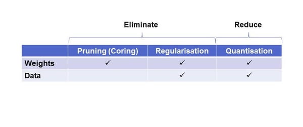
In any given network there will be two types of data flowing through the network, the weights (coefficients) and the ‘activation’ data that’s being processed at any time. So what’s required is to, wherever possible, eliminate weights and data. A weight represents how much importance the neural network applies to features it recognises in the network as it builds up a picture through the various layers. Therefore, if a weight can be set to zero that path can be eliminated from the convolution, so it will be able to run faster. Going back to our compressed digital image analogy, this is like removing the redundant information in the image.

This process of elimination is done through two techniques; pruning and regularisation – and is followed by reducing the computational cost of what’s left behind, which is done through quantisation.

Pruning your network

The aim of pruning the network is to increase the level of sparsity in the weights. It can be seen as the removal of connections or setting weights to zero – the end effect is the same.

To successfully prune, it’s necessary to apply a ‘coring’ function that removes weights that do not significantly improve accuracy. There are two ways to approach this, which have the same effect but have a slightly different implementation. The first is that if the value of a weight is below a certain threshold then it is automatically set to zero, and thus eliminated. The second approach is to set a small percentage of weights to zero.
The key benefit of this stage is that once a weight has been set to zero, it is gone for good. However, while pruning is a good start, ultimately its blunt force approach means you will start to degrade the performance of the task in hand. What needs to be done to recover this performance is an additional training stage.

Distil and regularise
This is done through ‘distillation’ – the transferring of knowledge from one network to another network. We have the original, ‘uncompressed’ floating point network that has been trained for a given task and we compare this to our pruned network – with the intention that the ‘softmax’ output from the pruned network – as in, it’s accuracy – will match that of the original. We iterate between coring and retraining, to increase the level of accuracy.

We can also add regularisation terms, a key tool in Deep Neural network (DNN) training, which adds a constraint that the trained network has a preference for zeros.

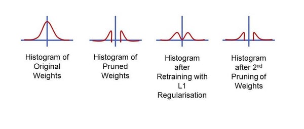
In the graph below you can see an illustration of the original weights, compared to the pruned version, and then how it looks after L1 Norm regularisation and further pruning. So after eliminating data and operations of the data that is left, how can we reduce the cost of those?
This is done by reducing the number of bits per weight. We start off with weights at a full precision 32-bit float. We can set a target bit-depth and rerun the training, applying quantisation to a randomly selected subset of the weights. This means that over time we are pushing the weights to quantised values and allowing the network to adapt to this. Eventually, we can clamp the weights to their nearest quantised values.

Choosing to target bit-depths lower than 32-bits will provide a significant reduction in your energy per inference, especially if you’re able to go down to as low as 4-bit, should your chosen hardware platform support it.

As a case in point, our recently announced PowerVR Series2NX NNA natively supports these low bit-rates, down to as low as 4-bits and also ‘exotic’ bit-rates such as 5-bits, which differentiates it from conventional DSPs and competing neural network accelerators. Note that the data is packed and optimally stored in memory on the NNA and while the internal pipeline is high-precision, it supports variable bit-depths on a per layer basis, so you can really optimise the training to maximise efficiency and accuracy.

When training, the developer can choose to quantise to the same bit-depth as the weights or to have more or less precision for activations than weights. It may well be worth having more bits for your data activations than for your weights.
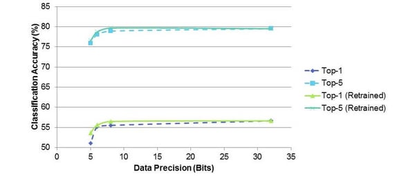
What you can see in the above is that when increasing the level of sparsity to 90%, retraining is highly beneficial to ensure the Top 5 classification accuracy remains high. Looking at the quantisation of the weights from 32-bit sweeping down to 5-bit, we can see you can drop to as low as 8-bit without much loss of performance without having to retrain, but to move below this, which is what you’ll want for an embedded device, retraining provides great benefits.

Conclusion
As we can see, optimising neural networks for efficient inferencing is not a trivial task, but can provide significant benefits, in terms of bandwidth reduction and therefore power consumption. The workflow tools included with PowerVR Series2NX NNA, abstract this complex task and providing a one-step process for fast prototyping of neural network powered applications. However, tuning and optimisation using the methods described in this post will enable you to make the best use of the hardware you’re running on, which is vital when targeting mobile and embedded platforms.

While this could be a GPU, a dedicated accelerator such as the Series2NX will provide performance that is orders of magnitude faster, making it the only neural network accelerator IP available on the market that can deliver the level of performance needed to make tomorrow’s powerful next-generation AI and vision-based applications run effectively within mobile power envelopes.

To keep up with further news on PowerVR and our NNA you can follow us on Twitter, Twitter @ImaginationTech.