- 25 May 2021
- Szabolcs Csefalvay
A major challenge for fast, low-power inference on neural network accelerators is the size of the models. There is a trend in recent years towards deeper neural networks with more activations and coefficients, and with this rise in model size, comes a corresponding rise in inference time and energy consumption per inference. This is particularly significant in resource-constrained mobile and automotive applications. Low-precision inference helps reduce inference cost by reducing DRAM bandwidth (which is a significant contributor to device energy consumption), compute logic cost and power consumption.
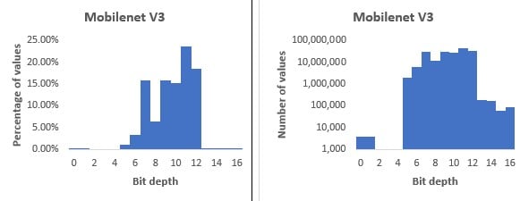
In this context, the following question naturally arises: what is an optimal bit depth at which to encode neural network weights and activations? There are several proposed number formats that reduce the bit depth, including Nvidia’s TensorFloat , Google’s 8-bit asymmetric fixed point (Q8A) and bfloat16 . However, while being a step in the right direction, these formats cannot be said to be optimal: for example, most of these formats store an exponent for each individual value to be represented, which can be redundant when multiple values share the same range. More importantly, they do not consider the fact that different parts of a neural network often have different bit-depth requirements. Some layers can be encoded with a low bit depth, while other layers (like input and output layers) need a higher bit depth. An example of this is MobileNet v3, which can be converted from 32-bit floating point to bit depths mostly in the 5-12 bits range (see Figure 1).
We call using different bit depths to encode different parts of the original floating-point network variable bit depth (VBD) compression.
There is of course a trade-off between the bit-depth of weight encoding and network accuracy. A lower bit-depth results in more efficient inference, but removing too much information will damage accuracy, meaning there is an optimal trade-off to be found. The goal of VBD compression is to balance the trade-off between compression and accuracy. A principled approach is to treat it as an optimisation problem: we want a network that achieves the best possible accuracy with as few bits as possible. This is achieved by adding a new term to the loss function that expresses the cost of network size so that it can be minimised along the original loss function, which informally can be written as:
total loss=network error+γ(network size)
where γ is a weighting factor that governs the target trade-off between network size and error.
To compress a network this way we, therefore, need two things: a differentiable measure of accuracy (error), and a differentiable measure of network size (compression bit depth). Differentiability of both the network size term and the network error term with respect to the number of bits is vitally important because it allows us to optimise (learn) the bit depths.
Differentiable network size
For differentiable quantisation, we can use any function with a differentiable bit-depth parameter that maps one or more floating-point values to a hardware-representable compressed number format. For example, we could use a variable bit-depth version of Google’s Q8A quantisation (where the representable range is not centred at zero):
![]()
Where:
- ⌊x⌉ is x rounded to the nearest integer (using the rounding mode of the target hardware platform)
- B is the bit depth.
- E is an exponent of a floating-point representation.
- α is the asymmetry parameter.
In practice, quantisation parameters B, E and α are used to compress multiple weights, e.g., a single parameter is used to compress an entire neural network layer (activation or weight tensor) or a channel within a layer.
We can also use symmetric quantisation (effectively to a scaled B-bit unsigned integer format), by setting the asymmetry parameter to 0:
![]()
To enable backpropagation to all parameters we use the Straight-Through Estimator by overriding the gradient of the round function as 1. This makes all operations in the formula differentiable, making all parameters, including the bit depths, learnable!
At this point we have a choice of which parameters to train:
- Both weights and bit depths for maximum compression.
- Only the weights and exponents (for a fixed bit depth).
- Only the quantisation parameters, which has several benefits (discussed below) at the cost of a potentially lower compression ratio.
Option 3 was chosen when producing the results in this article.
Another aspect to consider is the optimisation of the bit-depth parameter B (and for some formats the exponent E): any hardware would require B to be an integer. To find an integer solution we have multiple choices:
- To apply rounding with the straight-through estimator to the B parameter as well (e.g., using the formula
 . However, this introduces a discontinuity to the optimisation surface that, although possible to handle, is beyond the scope of this article.
 - An alternative chosen here is to optimise B as a floating-point value in the first stage of training, “conservatively” round it up to the nearest integer as ⌈B⌉ (otherwise important parts of the activation and weight tensors might get clamped), fix it as a constant and continue training. This loses about 0.5 bits of potential compression on average but guarantees that no inappropriate clipping takes place.
Differentiable measure of accuracy
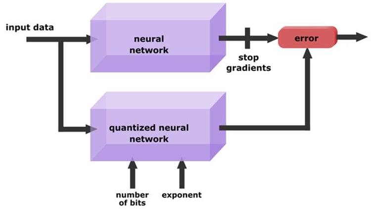
For measuring the accuracy of the network, we could simply use the same loss function the network was originally trained on. However, in many applications, the goal is to compress a network that was already trained in 32-bit floating point, which means we can use distillation loss instead. This means the compressed network’s accuracy is measured against the original network’s output. In this work, the absolute difference between (the output) logits was chosen as the distillation loss, but other measures are also possible.
Formally, the distillation loss used is defined as:
![]() (eq. 1)
(eq. 1)
Figure 2 illustrates this.
Distillation loss has many advantages:
- Label-free training: We do not need labelled data to compress a network, since we replaced labels with the output of the original network. This means we can compress a network without access to the (possibly proprietary) original dataset: we only need representative inputs and the original network.
- Generality: The neural network compressor can be defined universally; it doesn’t need to be network-specific.
- Less training data: Since we’re only training the quantisation parameters, the scope for overfitting is significantly reduced, so we can use much less training data. Sometimes even one image is enough!
- Soft targets: Since distillation loss derived from an input contains more information about the quantisation error than a label does, it allows for faster and more accurate convergence.
- We can train the weights together with quantisation parameters using distillation loss. However, in that case, we need much more training data to prevent overfitting. A best-of-both-worlds approach is to train weights with a very small learning rate and stopping early. This way the weights can offset quantisation error without overfitting to the dataset.
Differentiable compression
Combining a universal, differentiable measure of accuracy with differentiable quantisation leads to a loss function for differentiable compression:
![]() (eq. 2)
(eq. 2)
where the first term is the error, and the second term is the cost in network size. B is the average bit-depth of the network, which can be calculated from the depth parameters throughout the network:
![]() (eq. 3)
(eq. 3)
Where c_i is the number of network parameters (weights or activations) quantised using bit-depth parameter B_i. Note that this measure depends on batch size. If the network is evaluated on batches of 32 for example, then the size of the activation tensors are effectively weighted 32 times higher than using a batch size of 1. If the goal is to store network weights in as little space as possible, activations can also be disregarded in this metric.
Choosing quantisation granularity
Some neural network representations, like Google’s Q8A format, allow different scale factors (related to exponents E above by a power of 2) to be applied to different channels of the weight tensors (filters). This finer granularity enables better network accuracy for a given compression level. The same goal can be achieved with variable bit-depth compression by applying separate E and α parameters for each channel while using the same B parameter for the entire tensor. Per-channel quantisation however leads to slower convergence, therefore in our experience it is faster to use a training stage that learns pre-tensor parameters, then break these up to per-channel parameters, and let them converge in another stage of training.
This finally leads to a three-stage training schedule:
- Train all quantisation parameters as per-tensor
- Switch to per-channel exponent and shift parameters
- Round bit-depths up to an integer and fix them to a constant, then train exponents and the shift parameter α. In addition, weights are also trained with a small learning rate.
Results
Object classification
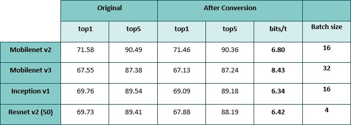
Accuracies of compressed classification networks. The Mobilenet v3 histogram in Figure 1 was the result of a different (shorter) training and was less compressed than the network in this table.
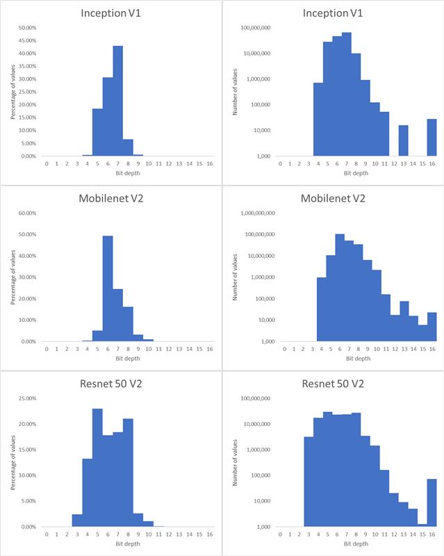
Histograms of bit-depths for select networks from this table are shown below.
Image Segmentation
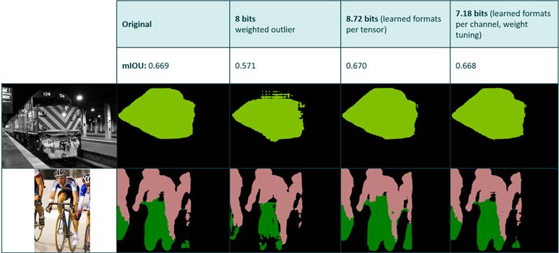
Comparison between different compression methods applied to a segmentation network. The second column is based on a heuristic that tries to determine the optimal exponents for a fixed bit depth without the use of backpropagation.
Style Transfer
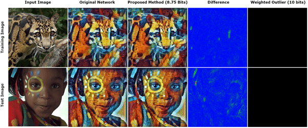
The last column gives an entirely blank output at 10 bits using the aforementioned heuristic.
Conclusion
Bit depths used for encoding neural network weights and activations have a significant effect on inference performance. Expressing the size-accuracy trade-off as part of the loss function makes it possible to learn optimal bit depths at arbitrary granularity during neural network training. In addition, when the optimisation assigns 0 bits to a part of the network it effectively removes that part from the architecture, serving as a kind of architecture search, reducing compute cost as well as bandwidth cost. Future work will explore this aspect of differentiable network compression.
We have presented a general and flexible method based on differentiable quantisation and distillation that allows the number of bits to be optimised for a wide variety of tasks without compromising accuracy. Our approach has several advantages, including short training times, reuse of a trained network, no need for labels, adjustable size-accuracy trade-off and a problem-agnostic loss function. In this way, we can compress networks to efficient variable bit depth representations without sacrificing fidelity to the original, floating-point network.
—
[i] https://blogs.nvidia.com/blog/2020/05/14/tensorfloat-32-precision-format/
[ii] https://www.tensorflow.org/lite/performance/quantization_spec
[iii] https://arxiv.org/abs/1905.12322
[iv] https://arxiv.org/abs/1308.3432
[v] https://arxiv.org/abs/1503.02531


